Ratio

Ratio:

Ratio : Number1:Number2

G column , we used GCD function =D4/GCD(D4,E4)&":"&E4/GCD(D4,E4)

H column , we used Text & Substitute Function =SUBSTITUTE(TEXT(D4/E4,"#/######"),"/",":")

Text function is suitable for negative number also, whereas GCD function is Not.

GCD function stands Greater common factor.
syntax : GCD(number1, [number2], ...)

Example: GCD(100,200) = 100
When you divide 100 by 100, its 1
& 200 by 100, its 2.

Since we need the ratio, by concatenate the results by using concatenate function or &":"&.

So, our formula returns as =D4/GCD(D4,E4)&":"&E4/GCD(D4,E4)

For H column Formula,  Using Text function TEXT(D4/E4,"#/######"), returns the result of maximum divided into the format "number1/number2". Example for if 100 is divided by 200, then text format will return 1/2 which is the maximum possible divide.
Since we need the result in 1:2 insteaed of 1/2, so we are using SUBSTITUTE function for it to substitute"/" by ":".

Our formula will be then,
=SUBSTITUTE(TEXT(D4/E4,"#/######"),"/",":")

Thanks

Split a number into integer and decimal portions.

Split a Number into Integer and Decimal portions.

For integer, you could also use formula =INT(D4). But since INT function is for only positive numbers. So, we are using here TRUNC function, =TRUNC(D4,0)

And for decimal , it is =MOD(D4,SIGN(D4))

Sequence of Months parallel to sequence of number.

Get Sequence of Months parallel to sequence of number.

In previous blog :
For sequence of number we used MOD function.
C4  =MOD(C3,12)+1

For, Sequence Month:
Formula: =TEXT(DATE(2000,C4,1),"mmm") in E4 cell.

Drag down the formula, you will get Months in series.
From Jan to Dec , then start jan to Dec and so on.

Repeate a Sequence of Number

To Repeat a sequence of number, we could use MOD function for it.
For Example , We need a column of sequence 1,2,3,4,5 and then start from 1,2,3,4,5 and so on..

For that use formula :
C4 = MOD(C3,5)+1, Where C3 is blank .
Drag down the formula ..

MOD function (MOD( number , divisor ) >> returns the remainder after a number is divided by a divisor. 
In our example 5 is the divisor, when number reaches to 5 in C9 cell  , it make it zero and since we are adding it with 1, our series again started it with one.

Thanks

Combine or Concatenate All Rows Data in One Cell !!

Combine All Rows Data in One Cell !!

Need to combine all Rows data in One Cell . Are you tired to use notepad for this for sure .

Here we have simple formula Itself in Excel to make your life easy :

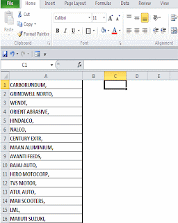
Let's Begin: Below Image is the Example:




Here's the Steps for it :

Step 1: 
Put Formula :
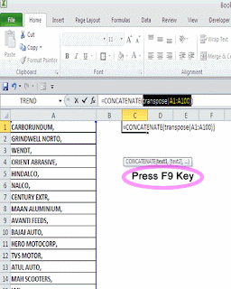
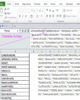
=CONCATENATE(transpose(A1:A100)) in formula bar, but DO NOT Press ENTER key. Instead Select transpose(A1:A100) and press F9. As Shown in below image. Once you pressed F9, Remove array ({,} this sign is in the beginning and in the end of transpose function) from Transpose function. See below image for reference.





Finally :

After removing Array then click Enter ,

Here we get the result .

Thank You!!

Have a Nice Day !!

Get All File-Names from Folder in Excel Spreadsheet !!

Get All File-Names from Folder in Excel Spreadsheet !!

It's very simple way to get all file-names from folder.

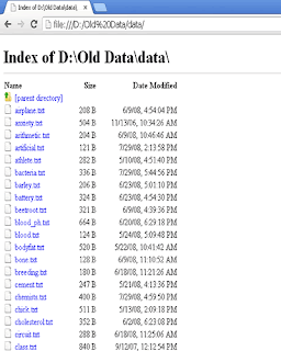
Below Image Shows All the File-Names that we want to Extract in Excel sheet :

Here is the Steps:

Step 1

 Open Browser (Any). In Example Google Drive  is opened . Placed file path as shown below image and open it.

 

Step 2 :
Once File opened in Google Drive as Above Image . Select Ctrl+A and Copy Ctrl+C

Step 3 :
Then, Open Excel Spreadsheet , Right-Click and Paste Special as Text

And here we go , 

Thank You !!

Have a Nice Day !!

Formula to link all the File Names in Excel.

Formula to link all the File Names in Excel:

You have the list of file-names,  and you want to link all the files to their destined path so that you can easily explore it just by clicking file-name on Excel Sheet instead always go to destined path and check file from there.

Here is the simple way,

Example: Below Image shows the list of file-name (which is static) in excel sheet (Sheet1) and what we want is when we click the file name , it opens from the destined path ("C:\sample"):

Here is the formula ,

=HYPERLINK("C:"&"\sample"&"\"&Sheet1!A2&".txt",Sheet1!A2) , drag down formula in sheet 2 and when you click it , i will open the file like below image.

Formula Explanation: 

• HYPERLINK(link_location,[friendly_name])  >>> 

1. Link_location is link to the destined path which is  -"C:"&"\sample"&"\"&Sheet1!A2&".txt"    >>> means Concatenate Destined path (you can also use Concatenate function) .
2. [friendly_name] >>> Name which you want to give and it will display in the cell. If ignore, the it will show the file path address (Example: C:\sample\1.txt). But if you define like we define Sheet1!A2, which shows file-name as shown in image above.

Thank You!!

Have a Nice Day !!